Physics and Machine Learning
Solver Agent: an Agentic AI Framework for Theoretical Physics Computations
We introduce Solver Agent, an AI framework based on large language models for calculations and proofs in mathematics and theoretical physics. I refer to the Github page for the instrunctions to how to install it. Applying Solver Agent, we study global F-theory uplifts of Type IIB orientifolds and their S-fold generalizations.
Demo of Solver Agent
The solution process is recorded in a persistent, append-only ledger, forming a directed dependency graph. Independent verification agents re-examine this ledger before returning a final answer, yielding an auditable and reproducible proof. The framework exports these sessions as a raw ledger.json, a human-readable report.html, and a printable report.tex.
Prompt 1
Count the number of \(\mathbb{Q}\)-terminal singularities in the weighted projective spaces \(\mathbb{P}^3_{[w_1,w_2,w_3,w_4]}\), for
Result 1
Interpret \(\mathbb Q\)-terminal as terminal on the \(\mathbb Q\)-factorial weighted projective threefold. At a coordinate point of weight \(r\), the local chart is the cyclic quotient \(\frac1r(a,b,c)\), where \(a,b,c\) are the other three weights modulo \(r\). Such an isolated quotient is terminal exactly when
Because the first two weights are \(1\), singularities can only occur on \(x_1=x_2=0\). If \(\gcd(w_3,w_4)>1\), this whole coordinate line is singular; no point on it is terminal because terminal threefold singularities are isolated.
The classification is:
| Weights | Relevant singularities | Terminal points | Count |
|---|---|---|---|
| \((1,1,2,2)\) | singular coordinate line since \(\gcd(2,2)=2\) | none | \(0\) |
| \((1,1,1,3)\) | \(\frac13(1,1,1)\), with age \(1\) for \(k=1\) | none | \(0\) |
| \((1,1,2,3)\) | \(\frac12(1,1,1)\), \(\frac13(1,1,2)\) | both | \(2\) |
| \((1,1,2,4)\) | singular coordinate line since \(\gcd(2,4)=2\) | none | \(0\) |
| \((1,1,3,4)\) | \(\frac13(1,1,1)\) fails; \(\frac14(1,1,3)\) passes | \(\frac14(1,1,3)\) | \(1\) |
| \((1,1,3,5)\) | \(\frac13(1,1,2)\) passes; \(\frac15(1,1,3)\) has age \(1\) | \(\frac13(1,1,2)\) | \(1\) |
| \((1,1,4,6)\) | singular coordinate line since \(\gcd(4,6)=2\) | none | \(0\) |
Hence, in the order asked,
and the total number of terminal singular points across all seven spaces is
Prompt 2
For each of the \(\mathbb{Q}\)-terminal geometries in the list, write the local group corresponding to the \(\mathbb{Q}\)-terminal singularities.
Result 2
Let \(P_i\) denote the coordinate point where only \(x_i\neq0\), and let \(\zeta_r=e^{2\pi i/r}\). At a weight-\(r\) coordinate point, the local model is \(\mathbb C^3/\mu_r\), with \(\mu_r\) acting with exponents given by the other three weights modulo \(r\).
The weighted projective spaces containing terminal singularities and their local groups are:
-
\(\mathbb P(1,1,2,3)\):
\[ P_3=[0:0:1:0]:\quad \frac12(1,1,1),\qquad \Gamma_{P_3}=\mu_2=\langle\operatorname{diag}(-1,-1,-1)\rangle; \]\[ P_4=[0:0:0:1]:\quad \frac13(1,1,2),\qquad \Gamma_{P_4}=\mu_3=\langle\operatorname{diag}(\zeta_3,\zeta_3,\zeta_3^2)\rangle. \] -
\(\mathbb P(1,1,3,4)\):
\[ P_4=[0:0:0:1]:\quad \frac14(1,1,3),\qquad \Gamma_{P_4}=\mu_4=\langle\operatorname{diag}(i,i,i^3)\rangle. \] -
\(\mathbb P(1,1,3,5)\):
\[ P_3=[0:0:1:0]:\quad \frac13(1,1,2),\qquad \Gamma_{P_3}=\mu_3=\langle\operatorname{diag}(\zeta_3,\zeta_3,\zeta_3^2)\rangle. \]
Thus, as abstract groups, the four terminal local groups are \(\boxed{\mu_2,\mu_3,\mu_4,\mu_3}\), with the diagonal representations above. The other four weighted projective spaces in the list have no terminal singular points.
Type IIB Compactifications on Calabi-Yau Orientifolds
The construction of Calabi-Yau orientifolds for Type IIB compactifications with fluxes requires geometric data for string theory models. We compute divisor topologies, fixed-point loci, and intersection numbers to classify and analyze \(O3/O7\) orientifolds arising from favorable Calabi-Yau threefolds [1-11].
Calabi-Yau Hypersurface in Toric Ambient Space
A toric ambient space \(\mathcal{A}\) of dimension \(d\) constitutes a complex algebraic variety containing an algebraic torus \(T \simeq (\mathbb{C}^*)^d\). One constructs this space via \(k\) homogeneous coordinates \(x_i\) as \(\mathcal{A} \simeq (\mathbb{C}^k \setminus Z)/(\mathbb{C}^*)^r\), where \(r = k - d\) defines the rank of the toric variety and the dimension of the Picard group. The torus \(T\) establishes a lattice \(N = \text{Hom}(\mathbb{C}^*, T) \simeq \mathbb{Z}^d\) and a dual character lattice \(M = \text{Hom}(T, \mathbb{C}^*) \simeq \mathbb{Z}^d\). The topological data of the toric variety lies within a fan \(\Sigma \subset N_\mathbb{R}\), a collection of strongly convex rational polyhedral cones intersecting along shared faces. The homogeneous coordinates \(x_i\) directly map to the rays \(\nu_i \in \Sigma\). The exclusion set \(Z\) is the zero locus of the Stanley-Reisner (SR) ideal, which eliminates coordinate combinations not sharing a common cone in the fan [12-14].
Constructing a Calabi-Yau threefold hypersurface \(X_3\) inside a toric ambient space maps the algebraic torus \(T\) to a polytope \(\Delta \subset M_\mathbb{R}\) and its dual \(\Delta^\circ \subset N_\mathbb{R}\). The normal fan \(\Sigma_\Delta\) captures the geometry by forming cones over the proper faces of \(\Delta^\circ\) with apexes at the origin. This normal fan defines a toric fourfold \(\mathcal{A}_{\Sigma_\Delta}\) containing the potentially singular Calabi-Yau hypersurface [13-18].
Smooth crepant resolutions translate to refining the normal fan \(\Sigma_\Delta\) into a simplicial fan \(\Sigma(\mathcal{T})\) via a Fine, Regular, Star Triangulation (FRST) \(\mathcal{T}\) of \(\Delta^\circ\). This triangulation produces a smooth ambient toric fourfold \(\mathcal{A} \equiv \mathcal{A}_{\Delta^\circ, \mathcal{T}}\) where a generic hypersurface emerges as the zero locus of a polynomial section of the anticanonical line bundle \(\mathcal{O}_\mathcal{A}(-K)\) [12, 15, 17, 19].
The non-trivial Hodge numbers of \(X_3\) derive from the polytope data [15]:
where \(l(\alpha)\) and \(l^*(\alpha)\) count the total and interior lattice points of a face \(\alpha\), respectively. For favorable Calabi-Yau manifolds, \(h^{1,1}(X_3) = h^{1,1}(\mathcal{A})\), allowing direct expansion of the Kähler form \(J\) in terms of the ambient toric divisors. The linear relations among the fan rays, \(\sum_i Q_i^a \nu_i = 0\), define the gauged linear sigma model (GLSM) charge matrix \(Q_i^a\), fixing a basis of divisors for \(H^{1,1}(\mathcal{A})\) that descends to \(X_3\) [20-21]. Intersection numbers \(\kappa_{abc}\) evaluate within the ambient fourfold \(\mathcal{A}\) by uplifting the integral via the first Chern class of the normal bundle, \(c_1(\mathcal{N}) = \sum_{i=1}^k D_i\):
Orientifolds and Tadpole Cancellation
The orientifold projection in Type IIB compactifications specifies an involution \(\iota\) acting on the Kähler form \(J\) and the holomorphic top form \(\Omega_3\), with the exact action depending on the choice of O-planes [2, 6, 22-23]:
This action splits the cohomology groups into even and odd eigenspaces under the pull-back of the involution. Following the analysis in [24-27], the dimensions of the complex structure eigenspaces satisfy:
The parameter \(S_O\) encodes the orientifold projection (\(S_O=+1\) for O3/O7-planes, \(S_O=-1\) for O5/O9-planes). The total Euler characteristic of the fixed loci, \(\chi_{\text{fix}}\), combines the Euler characteristics of codimension-one fixed surfaces \(S\) and isolated fixed points \(N_{O3}\) [4-5, 28-32]:
The D3-tadpole condition bounds the flux vacua [1-2, 4-6, 23, 33-42]:
Canceling the O7-tadpole requires introducing D7-branes on appropriate divisors. A non-rigid divisor allows recombination into a single Whitney umbrella [22, 43-49], whereas a rigid divisor requires placing an \(\text{SO}(8)\) stack (four D7-branes and four orientifold images) on top of the O7-plane locus [22, 36, 44, 50-53].
The geometric contribution from an \(\text{SO}(8)\) stack evaluates to [22, 33, 43, 54-56]:
Similarly, the geometric contribution from a Whitney umbrella (WU) is given by [44-47, 57]:
Divisor Topologies and Rigidity
Divisors dictating the brane configurations classify by their Hodge numbers \(h^\bullet(D) = \{h^{0,0}(D), h^{1,0}(D), h^{2,0}(D), h^{1,1}(D)\}\). A divisor \(D\) is rigid if it cannot continuously deform within \(X_3\), enforcing \(h^{2,0}(D) = 0\). A completely rigid divisor additionally requires \(h^{1,0}(D) = 0\), restricting all geometric moduli and Wilson lines. In contrast, rigid divisors with \(h^{1,0}(D) > 0\) form Wilson divisors, and non-rigid divisors lacking Wilson lines (\(h^{1,0}(D) = 0, h^{2,0}(D) > 0\)) classify as K3 divisors [4, 23, 50-51, 53, 58-77].
Evaluating \(h^\bullet(D)\) begins with topological quantities. The adjunction formula yields the Euler characteristic \(\chi(D)\) and arithmetic genus \(\chi_0(D)\) directly from the intersection numbers of \(X_3\):
These invariants determine \(h^{0,0}(D)\) and \(h^{1,1}(D)\) as functions of \(h^{1,0}(D)\) and \(h^{2,0}(D)\). Computing \(h^{1,0}(D)\) and \(h^{2,0}(D)\) requires resolving the Koszul exact sequence to map divisor cohomologies to line bundle cohomologies on the ambient toric space \(\mathcal{A}\). Specifically, the defining hypersurface short exact sequence induces a long exact sequence that splits in toric varieties, while the divisor exact sequence links these dimensions back to the divisor surface via Serre duality. Our computational framework utilizes cohomCalg to automatically evaluate these line bundle cohomologies on the ambient space.
Orientifold Classifications and F-theory Uplifts
Constructing an orientifold requires identifying the invariant fixed loci. A general geometric involution \(\iota\) maps coordinates via \(x_i \mapsto b_i x_{\rho(i)}\), combining a coordinate permutation \(\rho\) with a diagonal sign shift \(b_i\) [27, 31, 40, 61, 78-83].
Fixed loci classify into O7-planes (codimension-one), O5-planes (codimension-two), O3-planes (isolated points), and O9-planes (space-filling) [50-51, 84].
The involution determines the splitting of the Kähler moduli. The projection of the permutation matrix representation \(\mathbf{P}\) onto the Picard lattice defines \(\Lambda = \mathbf{Q}\mathbf{P}\mathbf{Q}^+\). The splitting is given by [27, 31, 79]:
F-theory Uplifts and Tadpole Corrections
Perturbative Type IIB orientifold compactifications admit a non-perturbative completion in F-theory [4, 9, 22, 28-29, 43, 48-49, 82, 85-86]. The compactification space is an elliptically fibered Calabi-Yau fourfold \(\pi: Y_4 \to B_3\), where the physical compactification base \(B_3 = X_3/\iota\) is the orientifold quotient of the Calabi-Yau threefold.
Sen's weak coupling limit connects the F-theory fourfold \(Y_4\) to the Type IIB orientifold \(X_3\). The elliptic fibration follows a Weierstrass model \(y^2 - x^3 - f x z^4 - g z^6 = 0\). The Type IIB seven-branes localize along the discriminant locus \(\Delta_W = 4f^3 + 27g^2 = 0\) [22, 28-29, 43, 87]. Parametrizing the sections \(f\) and \(g\) reveals that in the weak coupling limit \(c \to 0\), the discriminant locus factorizes:
The \(h^2\) component tracks the O7-plane locus in the base \(B_3\). Uplifting the remaining \(\eta^2 - h \psi = 0\) locus to \(X_3\) generates the recombined Whitney umbrella equation \(\eta^2 - x_S^2 \psi = 0\), explicitly canceling the O7-plane tadpole. When the O7-plane wraps a rigid divisor, the sections force the discriminant to vanish to degree six (\(\Delta \propto h^6\)). This configuration yields an \(I_0^*\) singularity characterizing an \(\mathrm{SO}(8)\) stack, where four D7-branes and four orientifold images stack precisely over the O7-plane [22, 44-45, 47].
The D3-brane tadpole condition in F-theory takes the form [33, 88]:
Defining \(N_{D3}/2 = \chi_{\text{st}}(Y_4)/24\) in F-theory already incorporates contributions from Type IIB O3-planes. The base \(B_3\) contains terminal quotient singularities from the orientifold quotient of O3-plane fixed points, inherited by the uplifted fourfold \(Y_4\). Naively extracting the Euler characteristic from the top Chern class misses these isolated singularities. The exact geometric formula computes the stringy Euler characteristic \(\chi_{\text{st}}(Y_4)\) via [31, 33, 44, 48, 84, 89-102]:
Results
In arXiv:2609.35958 [hep-th] we determine the stringy Euler characteristic \(\chi_{\text{st}}(\hat Y_4)\) of the Calabi-Yau fourfold \(\hat Y_4\) by incorporating contributions from the terminal quotient singularities of the base \(B_3\). The global stringy correction depends on the orders \(k_b \in \{2,3,4,6\}\) of the local cyclic groups at the singular points \(b\in\text{Sing}(B_3)\). Letting \(N_k\) denote the number of singularities of order \(k\) in \(B_3\), the total stringy Euler characteristic is
where \(\mathcal Y_4\) is the canonical smooth Deligne-Mumford stack associated with \(\hat Y_4\). The integral computes the Euler-Satake characteristic of the stack, and the sum captures the local stringy weight of each quotient singularity. This explicit expansion recovers \(\eqref{eq:Euler4fold}\) for pure O3-plane configurations, where \(N_{\text{O3}} = N_2\); the remaining terms capture the contributions from S-fold terminal quotient singularities.
These stringy corrections extend to vertical divisors \(\bar D = \pi^*D\) inherited from the base \(B_3\). The Euler-Satake characteristic of the induced stack divisor \(\mathcal D\) is given by the integral \(\int_{\mathcal D} c_3(T\mathcal D)\). Letting \(N_k(D)\) denote the number of order-\(k\) singularities lying on the divisor \(D\), the ordinary Euler characteristic \(\chi(\bar D)\) of the coarse divisor satisfies the Jefferson-Kim conjecture [31]:
The stringy Euler characteristic \(\chi_{\text{st}}(\bar D)\) of the vertical divisor requires a different local weight. The local McKay correspondence for the induced three-dimensional quotient singularities yields
Orientifold Database Generation
The Python scripts in this module automate the extraction of geometrical properties and tadpole data into a structured JSON database:
- generate_complete_orientifold_db_mixed.py: Queries a complete dataset of Calabi-Yau threefolds, computes valid orientifold involutions, evaluates O-planes, and extracts tadpole constraints across the geometries.
- generate_single_polytope_orientifold_mixed.py: Performs the identical evaluation of orientifolds and tadpole constraints for a single user-specified polytope.
- generate_trilayer_orientifolds.py: Computes the orientifold data specifically for Calabi-Yau threefold hypersurfaces defined by the trilayer polytope construction, where the F-theory uplift is constructed directly as a Weierstrass model over the toric orientifold quotient base.
The output JSON logs the Calabi-Yau geometry and its orientifold data. For each favorable Calabi-Yau threefold, the output records the base geometric properties: the polytope identifier (POLYID), Hodge numbers (h11, h21), points of the dual polytope (polytope_points), and geometric data for triangulations (triangulations).
The valid orientifold involutions are explicitly logged in the orientifolds list. Each entry records the geometric configuration and physical constraints governing the tadpole cancellation:
Basic Data & Involution
- TRIANGN and INVOLN: Indices specifying the triangulation and the involution orbit.
- INVOL: The string representation of the coordinate permutation \(x_i \to x_{P(i)}\).
- SCANON and BCANON: The canonical sign \(S_{\text{canon}} \in \{1, -1\}\) and a list of coordinate signs \(b_{\text{canon}} \in \{1, -1\}\) that define the diagonal sign shift.
- SOMEGA: The orientifold projection choice \(S_O\). Setting \(S_O = +1\) identifies an O3/O7-plane configuration, whereas \(S_O = -1\) identifies an O5/O9-plane configuration.
- is_reducible: Indicates whether the Calabi-Yau hypersurface vanishes identically under the orientifold equations.
- integer_hodge: Indicates if the equivariant Hodge numbers are strictly integers.
Equivariant Hodge Numbers
The splitting of the cohomology groups under the pull-back of the involution is evaluated using the projection of the coordinate permutation matrix onto the Picard lattice, defining \(\Lambda\).
- h11_plus and h11_minus: Evaluate the splitting of the Kähler moduli according to \(\eqref{eq:h11_pm}\).
- h21_plus and h21_minus: Determine the complex structure splitting under \(\eqref{eq:h21_plus}\), derived from the total Euler characteristic of the fixed loci.
O-Planes Data (OPLANES)
The OPLANES array enumerates the fixed O-planes resulting from the orientifold equations. Each entry specifies:
- OIDEAL: The coordinate constraints defining the fixed locus.
- ODIM and chi: The dimension and Euler characteristic of the fixed plane.
- For O7-planes, the data includes the self-intersection D3, the Chern intersection c2D, topological divisor cohomologies (h10, h20, h11), and boolean flags indicating whether the divisor is rigid or completely_rigid.
Tadpole and F-theory Data
The tadpole_data array structures the physical constraints required for flux compactifications across valid combinations of O7-plane configurations (e.g., Whitney Umbrella or SO(8) stacks).
- N_O3 and chi_O7_total: Count the isolated O3-planes and sum the Euler characteristics of the O7-planes, mapping to \(\eqref{eq:chi_fix}\).
- chi_D7: Evaluates the D7-brane Euler characteristic for the given configuration.
- N_D3: Computes the total fractional D3-charge bounding the flux vacua, corresponding to \(\eqref{eq:D3_tadpole}\).
- N_flux_frac and N_D3_mobile_max: Specify the fractional part of the gauge flux and the maximum integer number of mobile D3-branes.
- chi_Y4_corrected: Computes the total stringy Euler characteristic \(\chi_{\text{st}}(Y_4)\) of the associated F-theory fourfold, derived from the D3-charge \(12 \cdot N_{D3}\).
- chi_Y4_correction_O3 and chi_Y4_naive: Decompose \(\chi_{\text{st}}(Y_4)\) into the stringy correction \(6 N_{O3}\) and the naive top Chern class integral.
- nodal_singularities and n_S_df0: Evaluate the presence and count of isolated \(I_0\) singularities in the D7-brane configuration.
- ed3_instantons: Lists completely rigid divisors capable of wrapping ED3-instantons, alongside their Hodge numbers and vertical stringy Euler characteristics.
References
[1] Grana, "Flux compactifications in string theory: A Comprehensive review", Phys. Rept. (2006).
[2] Blumenhagen, "Four-dimensional String Compactifications with D-Branes", Phys. Rept. (2007).
[3] Douglas, "Flux compactification", Rev. Mod. Phys. (2007).
[4] Denef, "Les Houches Lectures on Constructing String Vacua", Les Houches (2008).
[5] Weigand, "Lectures on F-theory compactifications and model building", Class. Quant. Grav. (2010).
[6] Ibanez, "String theory and particle physics: An introduction to string phenomenology" (2012).
[7] Maharana, "Models of Particle Physics from Type IIB String Theory and F-theory: A Review", Int. J. Mod. Phys. A (2013).
[8] Blumenhagen, "Basic concepts of string theory" (2013).
[9] Weigand, "F-theory", PoS (2018).
[10] Marchesano, "D-brane and F-theory Model Building" (2023).
[11] Marchesano, "The Standard Model from String Theory: What Have We Learned?", Ann. Rev. Nucl. Part. Sci. (2024).
[12] Cox, "Erratum to ``The Homogeneous Coordinate Ring of a Toric Variety''", arXiv e-prints (1992).
[13] Cox, "Toric varieties" (2011).
[14] William Fulton, "Introduction to Toric Varieties. (AM-131)" (1993).
[15] Batyrev, "Dual polyhedra and mirror symmetry for Calabi-Yau hypersurfaces in toric varieties", J. Alg. Geom. (1994).
[16] Kreuzer, "Complete classification of reflexive polyhedra in four-dimensions", Adv. Theor. Math. Phys. (2000).
[17] De Loera, "Triangulations: Structures for Algorithms and Applications" (2010).
[18] Reid, "Decomposition of toric morphisms" (1983).
[19] Altman, "A Calabi-Yau Database: Threefolds Constructed from the Kreuzer-Skarke List", JHEP (2015).
[20] Witten, "Phases of N=2 theories in two-dimensions", Nucl. Phys. B (1993).
[21] Hori, "Mirror Symmetry" (2003).
[22] Sen, "Orientifold limit of F theory vacua", Phys. Rev. D (1997).
[23] Giddings, "Hierarchies from fluxes in string compactifications", Phys. Rev. D (2002).
[24] Camara, "Flux induced SUSY breaking soft terms", Nucl. Phys. B (2004).
[25] Grana, "Soft supersymmetry breaking in Calabi-Yau orientifolds with D-branes and fluxes", Nucl. Phys. B (2004).
[26] Grimm, "The Effective action of N = 1 Calabi-Yau orientifolds", Nucl. Phys. B (2004).
[27] Crin\`o, "A database of Calabi-Yau orientifolds and the size of D3-tadpoles", JHEP (2022). arXiv:2204.13115 | GitHub Repository
[28] Morrison, "Compactifications of F theory on Calabi-Yau threefolds. 1", Nucl. Phys. B (1996).
[29] Morrison, "Compactifications of F theory on Calabi-Yau threefolds. 2.", Nucl. Phys. B (1996).
[30] Gendler, "Superpotentials from Singular Divisors" (2022).
[31] Jefferson, "On the intermediate Jacobian of M5-branes", JHEP (2024). arXiv:2211.00210
[32] Collinucci, "F-theory on singular spaces", JHEP (2015).
[33] Sethi, "Constraints on low dimensional string compactifications", Nucl. Phys. B (1996).
[34] Uranga, "D-brane probes", Nucl. Phys. B (2001).
[35] Marchesano, "MSSM vacua from flux compactifications", Phys. Rev. D (2005).
[36] Blumenhagen, "GUTs in Type IIB Orientifold Compactifications", Nucl. Phys. B (2009). arXiv:0811.2936
[37] Bena, "The tadpole problem", JHEP (2021).
[38] Braun, "$G_4$ flux", JHEP (2021).
[39] Plauschinn, "The tadpole conjecture at large complex-structure", JHEP (2022).
[40] Gao, "The LVS parametric tadpole constraint", JHEP (2022).
[41] Gra{\~n}a, "The tadpole conjecture in asymptotic limits", JHEP (2022).
[42] L{\"u}st, "The tadpole conjecture in the interior of moduli space", JHEP (2023).
[43] Sen, "F theory and orientifolds", Nucl. Phys. B (1996).
[44] Collinucci, "D-brane Deconstructions in IIB Orientifolds", JHEP (2009). arXiv:0805.1573
[45] Braun, "D7-Brane Motion from M-Theory Cycles and Obstructions in the Weak Coupling Limit", Nucl. Phys. B (2008).
[46] Aluffi, "Chern class identities from tadpole matching in type IIB and F-theory", JHEP (2009).
[47] Collinucci, "Four-modulus 'Swiss Cheese' chiral models", JHEP (2009).
[48] Collinucci, "New F-theory lifts", JHEP (2009). arXiv:0812.0175
[49] Aluffi, "New Orientifold Weak Coupling Limits in F-theory", JHEP (2010).
[50] Polchinski, "Dirichlet Branes and Ramond-Ramond charges", Phys. Rev. Lett. (1995).
[51] Gimon, "Consistency conditions for orientifolds and D-manifolds", Phys. Rev. D (1996).
[52] Cicoli, "Moduli Stabilisation for Chiral Global Models", JHEP (2012).
[53] Morrison, "Classifying bases for 6D F-theory models", Central Eur. J. Phys. (2012).
[54] Douglas, "Branes within branes", NATO Sci. Ser. C (1999).
[55] Green, "I-brane inflow and anomalous couplings on d-branes", Class. Quant. Grav. (1997).
[56] Minasian, "K theory and Ramond-Ramond charge", JHEP (1997).
[57] Braun, "G-flux in F-theory and algebraic cycles", Nucl. Phys. B (2012).
[58] Witten, "Nonperturbative superpotentials in string theory", Nucl. Phys. B (1996).
[59] Blumenhagen, "D-Brane Instantons in Type II Orientifolds", Ann. Rev. Nucl. Part. Sci. (2009).
[60] Blumenhagen, "A Note on Poly-Instanton Effects in Type IIB Orientifolds on Calabi-Yau Threefolds", JHEP (2012).
[61] Gao, "On Classifying the Divisor Involutions in Calabi-Yau Threefolds", JHEP (2013).
[62] Kachru, "De Sitter vacua in string theory", Phys. Rev. D (2003).
[63] Cicoli, "String cosmology: From the early universe to today", Phys. Rept. (2024).
[64] Katz, "Geometric engineering of quantum field theories", Nucl. Phys. B (1997).
[65] Blumenhagen, "Spacetime instanton corrections in 4D string vacua: The Seesaw mechanism for D-Brane models", Nucl. Phys. B (2007).
[66] Caraffi, "New Type IIB Poly-instanton Effects and Axion Quintessence" (2026).
[67] Blumenhagen, "Lifting D-Instanton Zero Modes by Recombination and Background Fluxes", JHEP (2007).
[68] Bianchi, "Magnetized E3-brane instantons in F-theory", JHEP (2011).
[69] Palti, "Supersymmetric Protection and the Swampland", JHEP (2020).
[70] Polchinski, "String theory. Vol. 1: An introduction to the bosonic string" (2007).
[71] Polchinski, "String theory. Vol. 2: Superstring theory and beyond" (2007).
[72] Katz, "Geometric engineering of N=1 quantum field theories", Nucl. Phys. B (1997).
[73] Diaconescu, "Three-dimensional N=2 gauge theories and degenerations of Calabi-Yau four folds", Nucl. Phys. B (1998).
[74] Morrison, "Non-Higgsable clusters for 4D F-theory models", JHEP (2015).
[75] Camara, "Flux-induced SUSY-breaking soft terms on D7-D3 brane systems", Nucl. Phys. B (2005).
[76] Gomis, "An Open string landscape", JHEP (2005).
[77] Jockers, "D-terms and F-terms from D7-brane fluxes", Nucl. Phys. B (2005).
[78] Moritz, "Orientifolding Kreuzer-Skarke" (2023). arXiv:2305.06363
[79] Hassfeld, "Calabi-Yau Orientifold Hypersurfaces and their F-theory Uplifts" (2026). arXiv:2606.19423 | GitHub Repository
[80] Altman, "Orientifold Calabi-Yau threefolds with divisor involutions and string landscape", JHEP (2022).
[81] Gao, "Applying machine learning to the Calabi-Yau orientifolds with string vacua", Phys. Rev. D (2022).
[82] Collinucci, "New F-theory lifts. II. Permutation orientifolds and enhanced singularities", JHEP (2010). arXiv:0906.0003
[83] Carta, "A landscape of orientifold vacua", JHEP (2020).
[84] Garc\'\i{}a-Etxebarria, "$ \mathcalN=3 $ four dimensional field theories", JHEP (2016).
[85] Vafa, "Evidence for F theory", Nucl. Phys. B (1996).
[86] Blumenhagen, "F-theory uplifts and GUTs", JHEP (2009).
[87] Bershadsky, "Geometric singularities and enhanced gauge symmetries", Nucl. Phys. B (1996).
[88] Becker, "M theory on eight manifolds", Nucl. Phys. B (1996).
[89] David R. Morrison, and Glenn Stevens, "Terminal Quotient Singularities in Dimensions Three and Four", Proceedings of the American Mathematical Society (1984).
[90] Anno, "Four-dimensional terminal Gorenstein quotient singularities", Mathematical Notes (2003).
[91] Dasgupta, "A Note on low dimensional string compactifications", Phys. Lett. B (1997).
[92] Dasgupta, "M theory", JHEP (1999).
[93] Batyrev, "Stringy hodge numbers of varieties with Gorenstein canonical singularities" (1997).
[94] Esole, "The Geometry of G$_2$" (2017).
[95] Esole, "Characteristic numbers of crepant resolutions of Weierstrass models" (2018).
[96] Esole, "Characteristic numbers of elliptic fibrations with non-trivial Mordell-Weil groups" (2018).
[97] Esole, "Euler Characteristics of Crepant Resolutions of Weierstrass Models", Commun. Math. Phys. (2019).
[98] Esole, "48 Crepant Paths to $\textSU(2)\!\times\!\textSU(3)$" (2019).
[99] Esole, "The Geometry of SO(3)" (2019).
[100] Esole, "USp(4)-models" (2019).
[101] Esole, "Flops and Fibral Geometry of E$_7$-models" (2020).
[102] Aluffi, "Chern classes of blow-ups", Math. Proc. Cambridge Philos. Soc. (2010).
Learning to Trace Seiberg Dualities
We apply machine learning methods to identify Seiberg dualities [1] between supersymmetric quiver gauge theories.
Seiberg Dualities in Quiver Gauge Theories
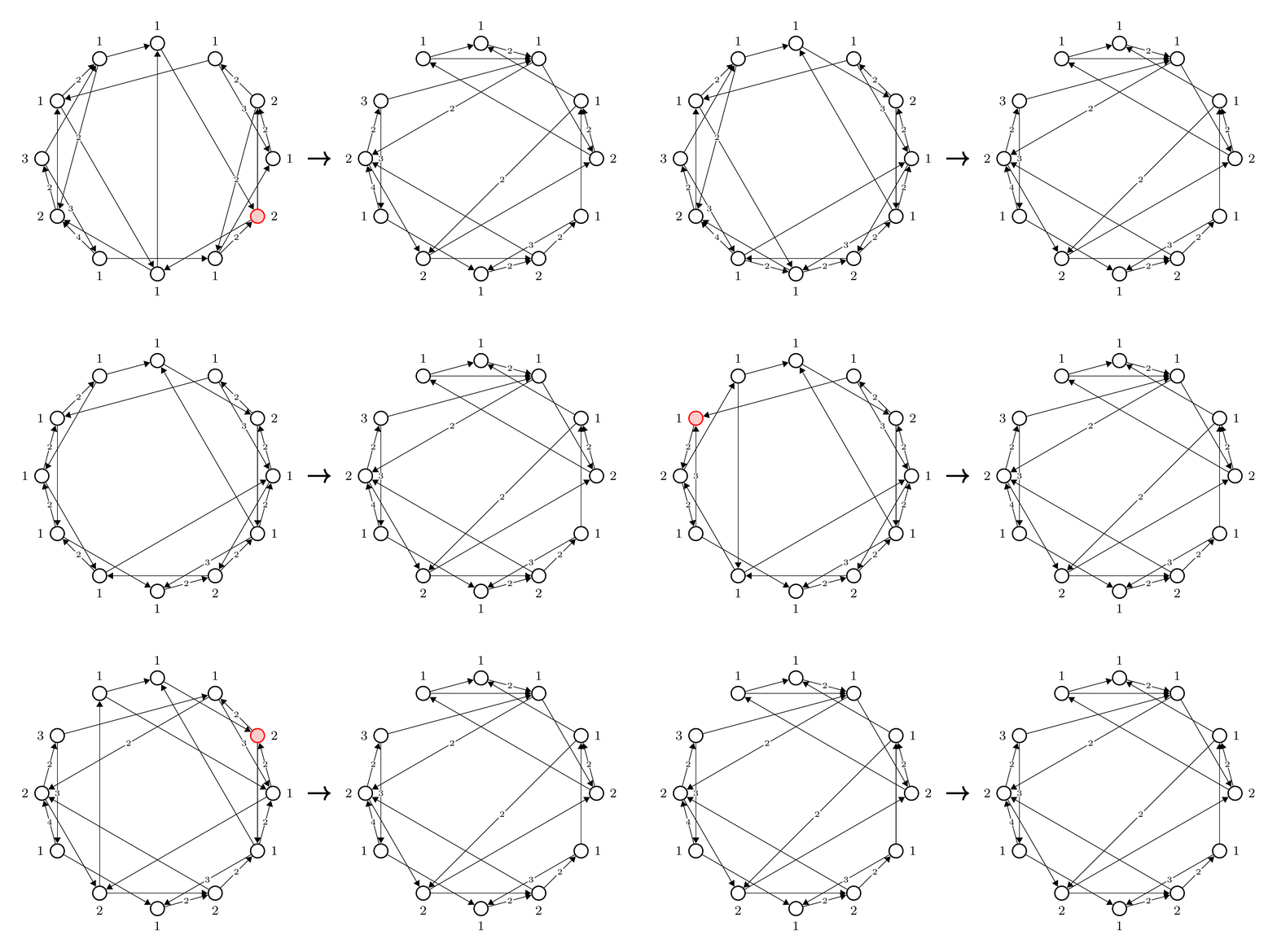
We consider 4D \(\mathcal{N} = 1\) quiver gauge theories with \(\text{SU}(N_i)\) gauge groups. The nodes represent gauge factors, and the directed arrows specify bifundamental chiral multiplets. The adjacency matrix \(\mathbf{A}\) defines the matter content. Anomaly cancellation requires the rank assignments to satisfy:
Seiberg duality operates locally on a single node \(k\). The mutation alters the gauge group rank to \(N_k' = \sum_j N_j A_{jk} - N_k\). All other ranks \(N_i\) for \(i \neq k\) remain unchanged. Connected arrows reverse direction. Mesonic fields generate new arrows \(A_{ik}A_{kj}\) between adjacent nodes \(i\) and \(j\), while oppositely oriented arrows annihilate.
The mutation of the adjacency matrix follows the Fomin-Zelevinsky rule [2, 3]:
where the net flow of arrows \(\Delta_{ij}\) from node \(i\) to node \(j\) is computed by adding the new mesonic arrows and subtracting any oppositely oriented arrows:
Chaining these simple duality operations produces a sequence of mutations \(Q^{(n)} = D_{j_n} \dots D_{j_1} Q\). The set of theories connected by these operations forms a duality tree [4-9]. Finding the exact sequence of dualizations connecting two distinct quiver gauge theories requires navigating this tree. We formulate this as a pathfinding problem where the quiver forms a state in a graph and mutations represent the edges. We developed two Graph Neural Networks (GNNs) [10, 11] to guide search algorithms through this space:
Pathfinders for Duality Sequences
We implement five search algorithms to find paths between related theories.
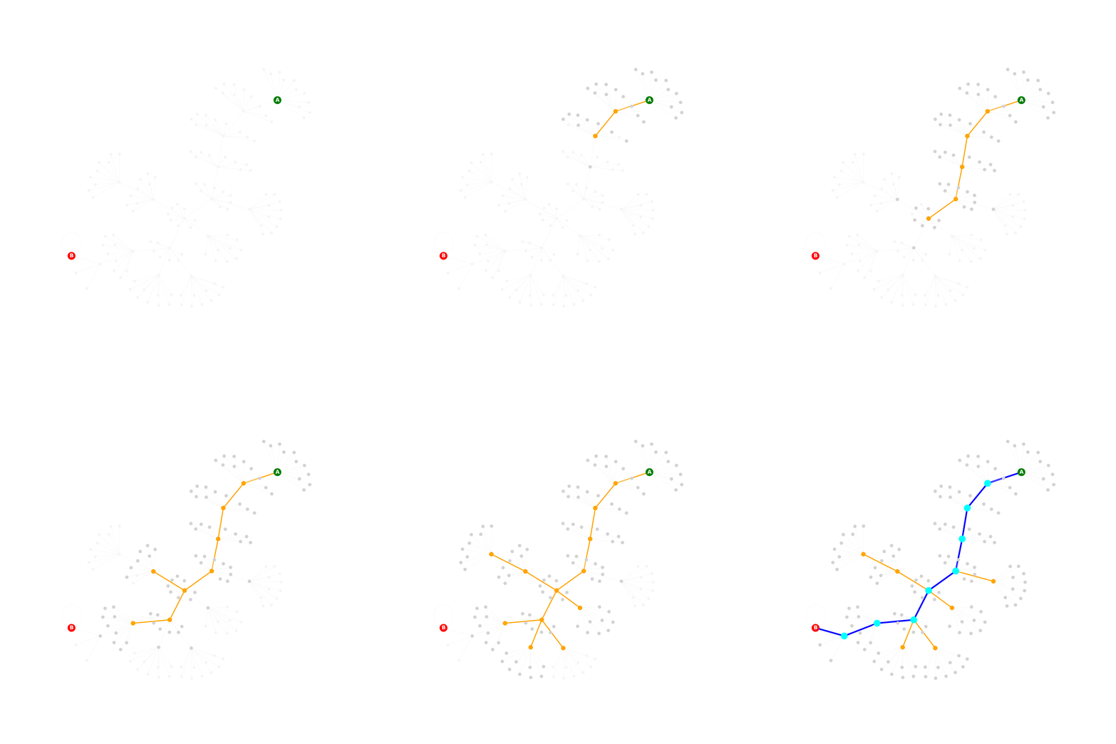
DGNN Pathfinder: A bidirectional A* search using the DGNN distance output as the heuristic function. The evaluation functions for the forward and backward frontiers are:
The step cost is fixed at \(g(Q_{n+1}) = g(Q_n) + 1\). The heuristic occasionally exhibits non-monotonicity, forcing the priority queue to explore uninformative branches and delaying convergence.
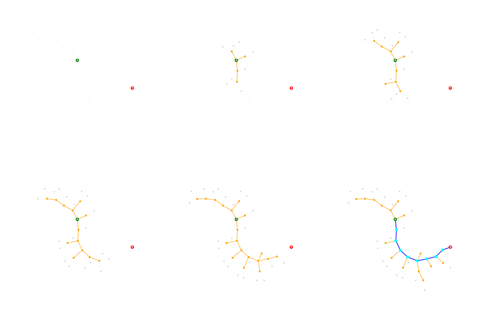
AGNN Pathfinder: A unidirectional beam search (\(B=3\)). It uses the AGNN mutation probability distributions to compute the path cost. The trajectory cost accumulates as:
Highly probable mutations contribute minimally to the cost, while unlikely ones heavily penalize the branch. The fixed beam width discards alternative branches and lacks a backtracking mechanism.
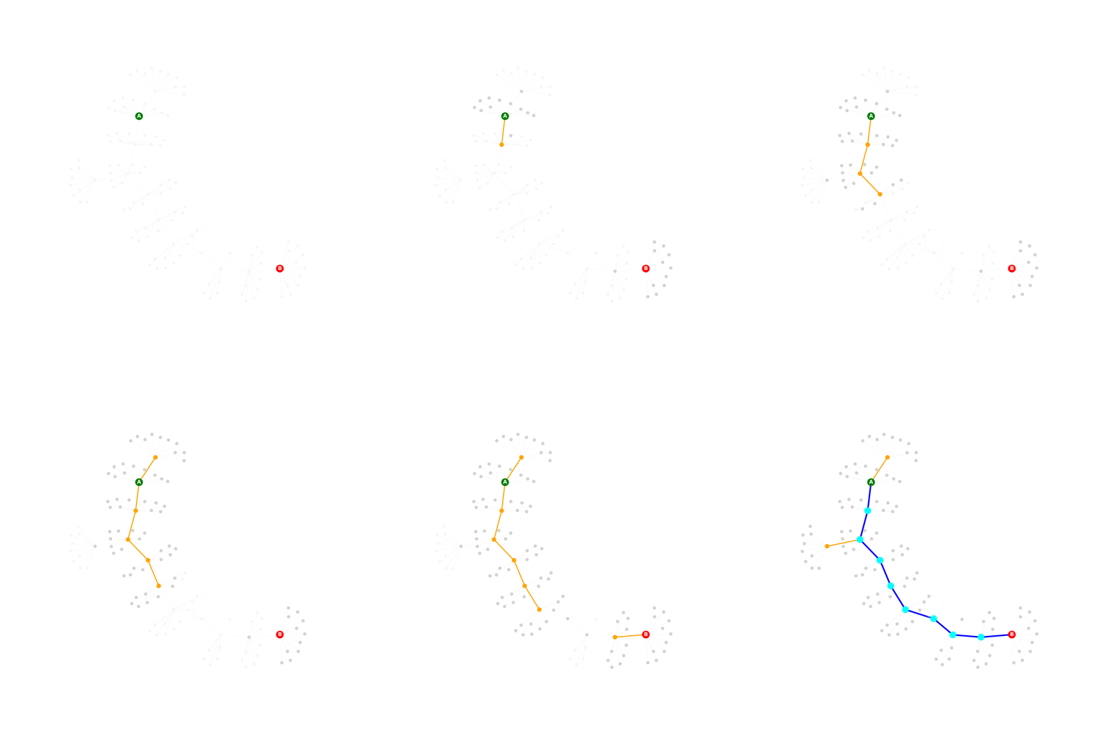
Hybrid Pathfinder: A bidirectional A* search combining DGNN distance estimates and AGNN branch probabilities. The cumulative trajectory cost updates recursively via:
The AGNN acts as a soft pruning mechanism, penalizing unlikely branches and preventing the algorithm from stalling in flat regions of the DGNN landscape.
LCA Pathfinder: A bidirectional A* search without neural network guidance. The cost function \(g(D_k)\) penalizes mutations based on gauge ranks (\(c_{\text{dec}}\) if rank decreases, \(c_{\text{eq}}\) if rank is unchanged, and \(c_{\text{inc}}\) if rank increases):
It forces both search trees toward simpler quivers to locate a Lowest Common Ancestor.
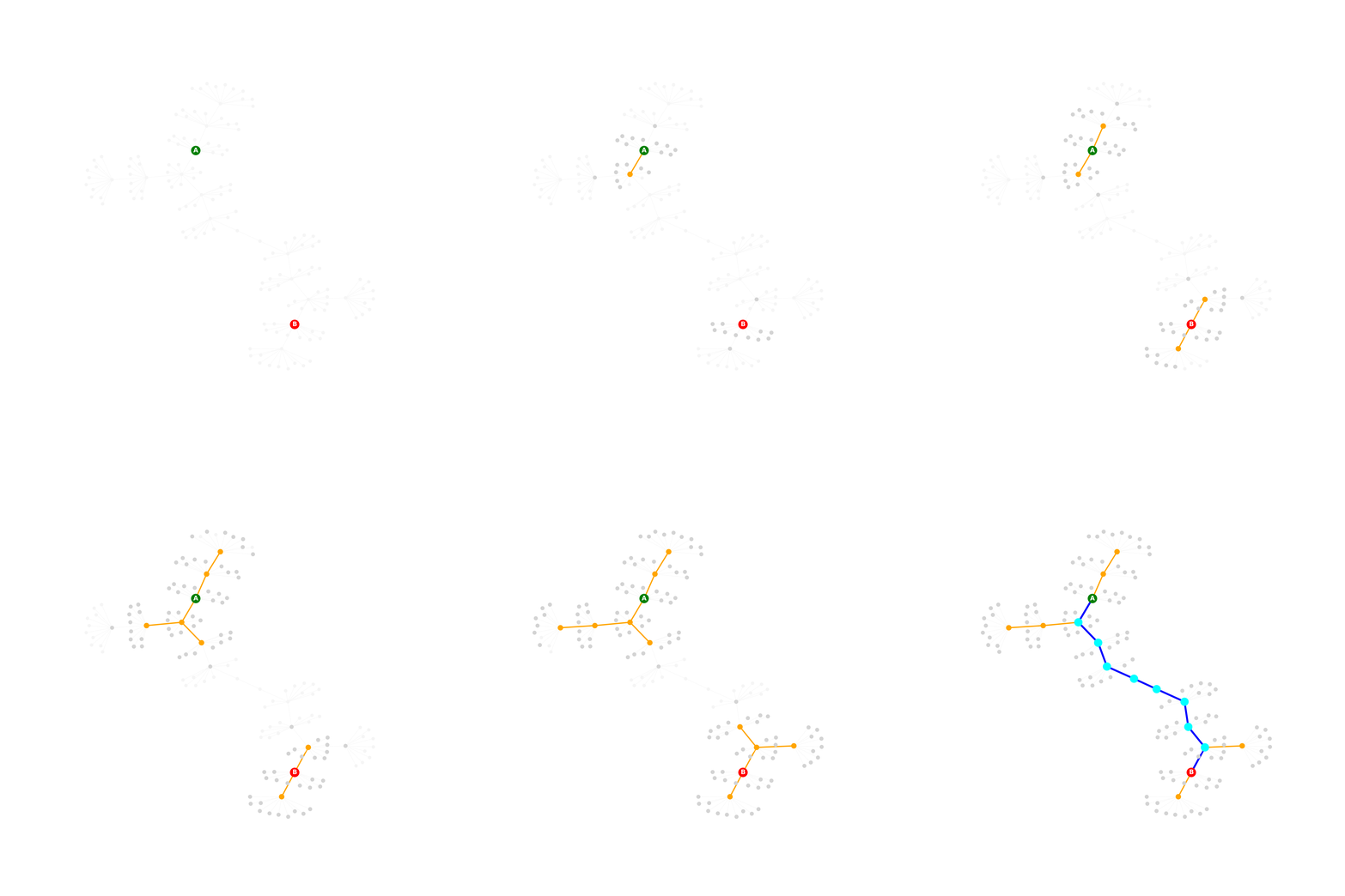
Hybrid LCA Pathfinder: Integrates the LCA rank penalties into the Hybrid pathfinder. The heuristic function incorporates a penalty proportional to the total rank:
This secondary penalty biases the search toward smaller-rank theories when network confidence is low.
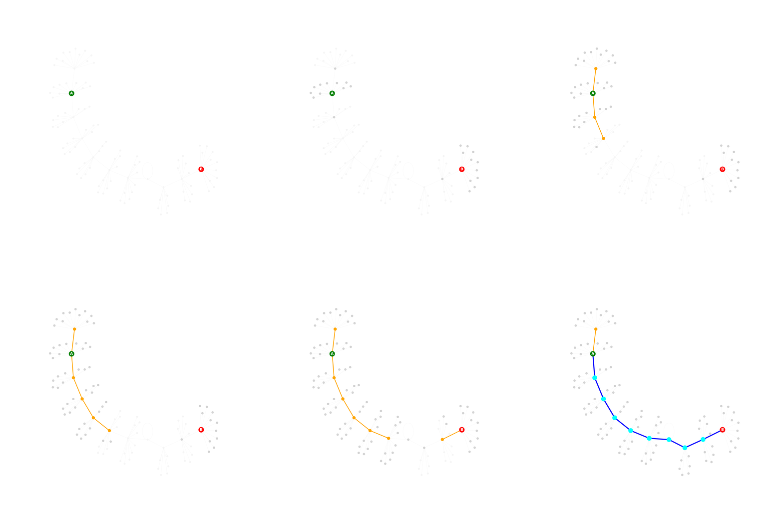
Results
We evaluate the pathfinder performances by averaging the metrics across all distances and node counts in each dataset. The Effective Efficiency Ratio (EER) multiplies the Success Rate (\(\overline{\text{SR}}\)) by the Efficiency Ratio (\(\overline{\text{ER}}\)). The first table compares the neural pathfinders against the uninformed Breadth-First Search (BFS) baseline. The second table compares them against the classical Lowest Common Ancestor (LCA) heuristic.
Performance vs BFS
| Data | Pathfinder | \(\overline{\text{SR}}\) (%) | \(\overline{\text{ER}}\) | \(\overline{\text{EER}}\) |
|---|---|---|---|---|
| ID | DGNN | \(99.94\) | \(430.25\) | \(429.99\) |
| AGNN | \(76.12\) | \(928.59\) | \(706.84\) | |
| Hybrid | \(100.00\) | \(790.08\) | \(790.07\) | |
| LCA | \(100.00\) | \(763.66\) | \(763.66\) | |
| OOD 1 | DGNN | \(99.51\) | \(134.38\) | \(133.72\) |
| AGNN | \(50.91\) | \(305.15\) | \(155.35\) | |
| Hybrid | \(99.84\) | \(221.99\) | \(221.63\) | |
| LCA | \(99.97\) | \(176.13\) | \(176.08\) | |
| OOD 2 | DGNN | \(99.34\) | \(714.42\) | \(709.74\) |
| AGNN | \(78.64\) | \(1175.18\) | \(924.21\) | |
| Hybrid | \(99.92\) | \(881.67\) | \(880.96\) | |
| LCA | \(100.00\) | \(568.25\) | \(568.25\) |
Performance vs LCA
| Data | Pathfinder | \(\overline{\text{SR}}\) (%) | \(\overline{\text{ER}}\) | \(\overline{\text{EER}}\) |
|---|---|---|---|---|
| ID | DGNN | \(99.94\) | \(0.83\) | \(0.83\) |
| AGNN | \(76.12\) | \(2.04\) | \(1.55\) | |
| Hybrid | \(100.00\) | \(1.10\) | \(1.10\) | |
| Hybrid LCA | \(100.00\) | \(1.14\) | \(1.14\) | |
| OOD 1 | DGNN | \(99.51\) | \(0.54\) | \(0.53\) |
| AGNN | \(50.91\) | \(1.03\) | \(0.52\) | |
| Hybrid | \(99.84\) | \(0.83\) | \(0.83\) | |
| Hybrid LCA | \(100.00\) | \(0.98\) | \(0.98\) | |
| OOD 2 | DGNN | \(99.34\) | \(0.83\) | \(0.83\) |
| AGNN | \(78.64\) | \(1.91\) | \(1.50\) | |
| Hybrid | \(99.92\) | \(1.16\) | \(1.16\) | |
| Hybrid LCA | \(100.00\) | \(1.18\) | \(1.18\) |
Overview of Search Algorithms
A* Search: An informed search algorithm that selects paths by minimizing the evaluation function \(f(n) = g(n) + h(n)\). The cost \(g(n)\) accumulates along the path, while the heuristic \(h(n)\) estimates the remaining distance. The algorithm maintains unexplored branches in a priority queue. This structure enables backtracking when a path reaches a dead end. Bidirectional A* accelerates the search by expanding forward from the initial theory and backward from the target theory simultaneously.
Beam Search: A greedy algorithm that limits memory overhead. It sorts generated candidate paths by cost and retains only the top \(B\) quivers at each depth step. The algorithm permanently discards all other branches. This reduces execution time but eliminates the ability to backtrack.
Graph Neural Network Architectures
We base our models on a Message Passing paradigm [10] combined with Graph Transformers [11, 12]. Nodes update their features by aggregating messages from their immediate neighborhood. We supplement this with global attention mechanisms to extract long-range topological data and prevent oversmoothing [13] in deep layers.
Distance GNN (DGNN): Estimates the scalar mutation distance between two quivers. The architecture uses a 3-layer GNN tokenizer with residual connections, followed by a 2-layer Transformer encoder. The fully activated node representation incorporates LayerNorm [14] and LeakyReLU [15] activations: \(\tilde{h}_i^{(\ell+1)} = \text{LeakyReLU}( \text{LayerNorm}( m_i^{(\ell+1)} ) )\). The network computes the element-wise absolute difference between the encoded nodes of both quivers, \(d_{\text{local}} = \frac{1}{K} \sum_{i=1}^K | h_{A,i} - h_{B,i} |\), concatenates this with global graph averages, and projects the result to a positive distance via a Multi-Layer Perceptron. We optimize the network using Mean Squared Error.
Adviser GNN (AGNN): Predicts the optimal first-step mutation. The initial feature vector encodes node ranks, incoming/outgoing arrows, and total adjacent ranks. The network adds Laplacian Positional Encodings (LPE) to distinguish structurally similar nodes. A Hybrid GPS encoder [11] yields dense nodes \(h_{A,i}\) and \(h_{B,i}\). An MLP classifier maps concatenated differences into unnormalized mutation scores (logits). The network applies a binary action mask \(\mathcal{M}\) to set scores for invalid mutations (e.g., those producing negative ranks) to negative infinity. A Softmax layer then normalizes the remaining scores into a valid probability distribution: \(P(D_i | Q_A, Q_B) = \text{Softmax}(\tilde{y})_i\).
Path Generation Script
The script pathfinders/find_path.py automates the search for Seiberg duality sequences between an initial and target quiver gauge theory. The output JSON structures the path details and search metrics.
The algorithm parses the starting and target graph data (ranks and adjacency matrices) and executes the selected search strategies.
Search Execution
The script runs multiple pathfinders sequentially based on command-line flags.
- --dgnn, --agnn, --hybrid, --lca, and --hybrid_lca trigger the respective search algorithms.
Path Output
The output records the specific mutation sequence.
- path contains the exact array of node indices mutated to connect the initial and target graphs.
- status confirms if the algorithm succeeded or encountered a dead end.
Search Metrics
The script records the number of explored nodes and outputs the search metrics.
- visited_states counts the total number of unique graph configurations generated and evaluated.
- meeting_depth_fwd and meeting_depth_bwd record the specific search depths where the two frontiers intersected in bidirectional algorithms.
References
[1] N. Seiberg, "Electric - Magnetic Duality in Supersymmetric Non-Abelian Gauge Theories", Nucl. Phys. B 435, 129--146 (1995), arXiv:hep-th/9411149.
[2] S. Fomin and A. Zelevinsky, "Cluster Algebras I: Foundations", (2001), arXiv:math/0104151.
[3] S. Fomin and A. Zelevinsky, "Cluster Algebras II: Finite Type Classification", Invent. Math. 154, 63--121 (2003), arXiv:math/0208229.
[4] S. Gukov, J. Halverson, F. Ruehle, and P. Su{\l}kowski, "Learning to Unknot", Mach. Learn. Sci. Tech. 2, 025035 (2021), arXiv:2010.16263.
[5] S. Franco, Y.-H. He, C. Herzog, and J. Walcher, "Chaotic Duality in String Theory", Phys. Rev. D 70, 046006 (2004), arXiv:hep-th/0402120.
[6] D. Berenstein and M. R. Douglas, "Seiberg Duality for Quiver Gauge Theories", (2002), arXiv:hep-th/0207027.
[7] C. P. Herzog, "Exceptional Collections and del Pezzo Gauge Theories", JHEP 04, 069 (2004), arXiv:hep-th/0310262.
[8] C. P. Herzog, "Seiberg Duality is an Exceptional Mutation", JHEP 08, 064 (2004), arXiv:hep-th/0405118.
[9] P. S. Aspinwall and I. V. Melnikov, "D-Branes on Vanishing del Pezzo Surfaces", JHEP 12, 042 (2004), arXiv:hep-th/0405134.
[10] J. Gilmer, S. S. Schoenholz, P. F. Riley, O. Vinyals, and G. E. Dahl, "Neural Message Passing for Quantum Chemistry", (2017), arXiv:1704.01212.
[11] L. Ramp{\'a}{\v{s}}ek, M. Galkin, V. P. Dwivedi, A. T. Luu, G. Wolf, and D. Beaini, "Recipe for a General, Powerful, Scalable Graph Transformer", (2022), arXiv:2205.12454.
[12] A. Vaswani, N. Shazeer, N. Parmar, J. Uszkoreit, L. Jones, A. N. Gomez, L. Kaiser, and I. Polosukhin, "Attention Is All You Need", NIPS 30, 5998--6008 (2017).
[13] X. Wu, A. Ajorlou, Z. Wu, and A. Jadbabaie, "Demystifying Oversmoothing in Attention-Based Graph Neural Networks", (2023), arXiv:2305.16102.
[14] J. Lei Ba, J. R. Kiros, and G. E. Hinton, "Layer Normalization", (2016), arXiv:1607.06450.
[15] A. L. Maas, "Rectifier Nonlinearities Improve Neural Network Acoustic Models", (2013).
Exploring Line Bundle Standard Models with Transformers
Heterotic Compactifications and Line Bundle Standard Models
We focus on finding \(\text{SU}(5)\) Grand Unified Theory (GUT) models from \(E_8 \times E_8\) heterotic string theory compactified on a Calabi-Yau threefold \(\mathbf{X}_3\) [1-7]. We associate a trivial line bundle to the hidden sector and require an equivariant vector bundle \(V\) that breaks the ten-dimensional gauge group into a split structure group \(H = \text{S}(\text{U}(1)^5)\) [8-10]. This breaks the observable \(E_8\) group down to \(G \times H = \text{SU}(5) \times \text{S}(\text{U}(1)^5)\).
We restrict \(V\) to be a direct sum of line bundles:
The integer vectors \(\mathbf{k}_a\) encode the first Chern classes expanded in the Kähler cone basis of \(\mathbf{X}_3\). To yield a consistent, supersymmetric vacuum, the bundle \(V\) must satisfy specific topological and physical constraints.
\(E_8\) Embedding: The line bundle sum must embed into \(E_8\), which imposes \(c_1(V) = \sum_{a=1}^5 \mathbf{k}_a = 0\). To prevent accidental isomorphisms that yield a non-unitary structure group and break the \(\text{SU}(5)\) GUT embedding, all proper subsets \(S \subset \{1,\ldots, 5\}\) must also satisfy \(\sum_{a \in S} \mathbf{k}_a \neq 0\) [11].
Anomaly Cancellation: We assume sufficient NS5-branes wrap effective curves to cancel the anomaly via the Green-Schwarz mechanism. This requires the curve \(c_2(T\mathbf{X}_3) - c_2(V)\) to be effective, imposing the bound:
Poly-Stability: The resulting effective field theory must be supersymmetric. The gauge connection on \(V\) must satisfy the Hermitian Yang-Mills equations at zero slope [12, 13]. For a direct sum of line bundles, this requires the slope \(\mu(L_a)\) of each individual line bundle to vanish simultaneously somewhere in the interior of the Kähler cone parameterized by the moduli \(t^i\):
The tensor \(\kappa_{ijk}\) denotes the intersection numbers of the Calabi-Yau threefold \(\mathbf{X}_3\).
Particle Spectrum: The spectrum must be chiral and contain exactly three families of multiplets in the \(\mathbf{10}-\overline{\mathbf{10}}\) representation. To achieve three chiral families upon quotienting the manifold by a freely acting discrete symmetry group \(\Gamma\), the index on the upstream covering space must scale with the group order [11, 14, 15]:
To prevent anti-generations and avoid Higgs color triplets that cannot be projected out by Wilson lines, the individual and pairwise indices must satisfy strict bounds [11, 14, 15]:
| Conditions | |
|---|---|
| \(E_8\) Embedding | \(c_1(V) = 0\,, \sum_{a\in S} c_1(L_a) \neq 0\) |
| Anomaly Cancellation | \(c_2(T\mathbf{X}_3) - c_2(V) \geq 0\) |
| Poly-Stability | \(\mu(L_a) = 0\) |
| Three Chiral Families | \(\text{ind}(V) = -3\vert\Gamma\vert\) |
| No Exotic Representations | \(-3\vert\Gamma\vert \leq \text{ind}(L_a) \leq 0\,, -3\vert\Gamma\vert \leq \text{ind}(L_a \otimes L_b) \leq 0\) |
Network Architecture and Reinforcement Learning
The search for vector line bundles is formulated as an autoregressive sequence generation task and solved using Proximal Policy Optimization (PPO) [16]. The objective is to construct the \(h^{1,1}(\mathbf{X}_3) \times 5\) matrix \(\mathbf{K}\) token-by-token. The first Chern class condition, \(c_1(V) = 0\), is imposed by construction by requiring that:
The remaining entries of \(\mathbf{K}\) are flattened in row-major order into a token sequence of length \(S = h^{1,1}(\mathbf{X}_3) \times 4\). The action space consists of integers \(a_t \in [0, 2k_{\text{max}}]\), which map to the sequence values via \(s_t = a_t - k_{\text{max}}\).
Actor-Critic Architecture: The policy and value functions are parameterized by a shared, decoder-only Transformer network [17]. Discrete input tokens map to dense vectors via a learnable embedding matrix, and we introduce a learnable positional encoding to break the permutation equivariance of the attention mechanism.
The input sequence is processed by \(L=4\) identical transformer blocks. Each layer applies a Masked Multi-Head Self-Attention (MHA) operation with \(H=8\) independent attention heads. The attention mechanism enforces causality via an upper-triangular mask. We apply a residual connection followed by Layer Normalization [18], and a Feed-Forward Network [19] with ReLU activation expands the dimensionality before projecting back down.
To predict the next action \(a_t\) and evaluate the current state, the model extracts the final hidden state vector \(h_t\) corresponding to the last processed token. This vector routes through two independent linear layers:
- Actor Head (Policy): Maps \(h_t\) to logits across the action space, converting them via a softmax activation into the probability distribution \(\pi_\theta(a_t | \mathbf{S}_t)\) for the next token.
- Critic Head (State-Value Estimate): Maps \(h_t\) to a scalar \(V_\theta(\mathbf{S}_t)\) predicting the expected cumulative reward for the sequence prefix.
Reward Shaping: The environment assigns a dense reward \(r_S\) only at the terminal step when the full vector bundle configuration is specified, evaluating the constraints using a composite scoring system:
- Triviality Masking: A binary mask zeros the final score if the bundle is degenerate.
-
Continuous Scoring: A continuous score is computed for each constraint using a log-barrier function:
\[ \begin{equation} S_{i, \text{cont}} = \frac{1}{1 + w_i \ln(1 + e_i)}\,. \label{eq:log_barrier_score} \end{equation} \]This range is constrained to \((0,1]\), preserving a gradient signal via the logarithm even for large errors that would otherwise suppress the reward. We define a continuous base score \(B = \sum_i w_i S_{i, \text{cont}}\) using uniform weights.
-
Perfection Bonus: A valid matrix satisfying all constraints receives an additive spike (\(+5\) bonus).
- Novelty Penalty: To avoid mode collapse into a single known solution, a rolling First-In-First-Out (FIFO) novelty buffer penalizes duplicates (under \(S_5\) permutation symmetry) by scaling down their reward by a penalty factor \(p_{\text{pen}} = 0.5\).
Synthesizing the triviality masking, the base score \(B\), the perfection bonus, and the novelty penalty, the terminal reward \(r_S\) assigned by the environment at step \(t=S\) for matrix \(\mathbf{K}\) is:
Because intermediate steps receive no immediate feedback, \(r_S\) is propagated backwards using Generalized Advantage Estimation (GAE) [20].
Complete Intersection Calabi-Yaus
Complete intersection Calabi-Yau (CICY) threefolds are algebraic varieties constructed as intersections of the zero loci of \(k\) homogeneous polynomials \(p_j\) in an ambient space \(\mathcal{A}\) [21]. This space is a product of projective spaces \(\mathbb{P}^{n_1} \times \dots \times \mathbb{P}^{n_m}\). The complex dimension of the threefold \(\mathbf{X}_3\) equals the dimension of \(\mathcal{A}\) minus \(k\). This yields the constraint:
A multi-degree \(q_j^i\) characterizes each polynomial \(p_j\), specifying the degrees in the homogeneous coordinates of each \(\mathbb{P}^{n_i}\). This information populates a configuration matrix:
The manifold \(\mathbf{X}_3\) is Calabi-Yau if the first Chern class of its tangent bundle \(c_1(T\mathbf{X}_3)\) vanishes. This imposes a condition on the polynomial degrees:
Each homogeneous polynomial \(p_j\) acts as a holomorphic section of a line bundle \(\mathcal{O}_{\mathcal{A}}(q_j)\) over the ambient space \(\mathcal{A}\). We define the normal bundle \(\mathcal{N}_{\mathbf{X}_3/\mathcal{A}}\) to \(\mathbf{X}_3\) as the direct sum of these \(k\) line bundles.
We restrict our analysis to favorable CICYs [22, 23]. In favorable geometries, the second cohomology group descends entirely from the ambient space. This means the restriction map \(\iota^* : H^2(\mathcal{A}, \mathbb{Z}) \to H^2(\mathbf{X}_3, \mathbb{Z})\) is surjective, leading to \(h^{1,1}(\mathbf{X}_3) = h^{1,1}(\mathcal{A}) = m\).
The basis of divisors \(J_i\) on \(\mathbf{X}_3\) corresponds to the pullback of the ambient hyperplanes. We expand the K\"ahler form on \(\mathbf{X}_3\) as \(J = t^i J_i\), with positive K\"ahler moduli \(t^i\). We define the triple intersection numbers \(\kappa_{abc}\) as:
The integral factorizes over the \(\mathbb{P}^{n_i}\) components of \(\mathcal{A}\). It evaluates to a non-zero value only when the integrand contains the exact volume form of \(\mathbb{P}^{n_i}\) for every factor.
Using the divisors \(J_i\), we calculate the total Chern class of \(\mathbf{X}_3\) via adjunction:
The adjunction formula allows us to compute the Euler characteristic of \(\mathbf{X}_3\) and extract the dimension \(h^{2,1}(\mathbf{X}_3)\) for favorable configurations.
Results
LB-Explorer evaluated ~50 favorable CICYs with \(h^{1,1}(\mathbf{X}_3) \in [4,15]\) and \(|\Gamma| \in [2,4]\). The pipeline ran across five seeds for 10 million episodes per geometry. The system filters the final solution sets to impose equivariant structure.
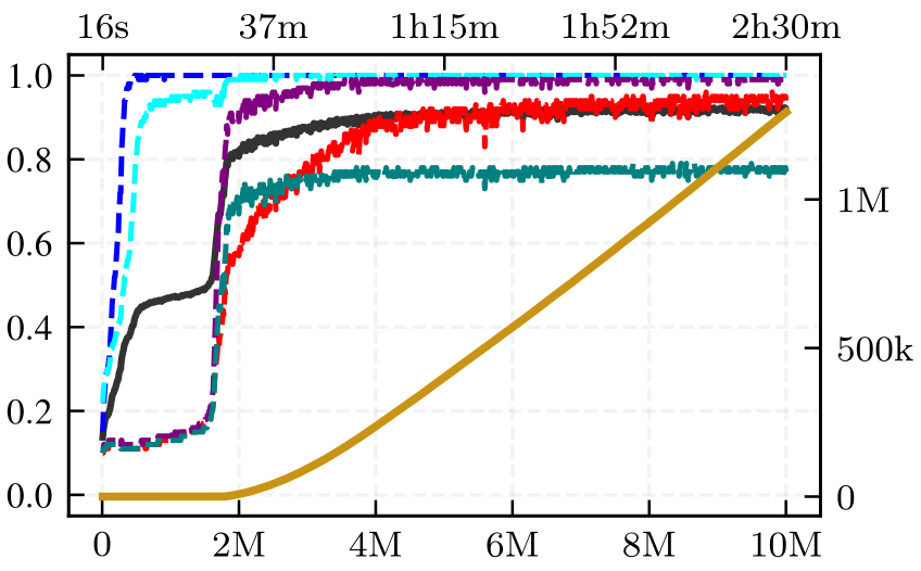
Staged Discovery
The neural network learns constraints sequentially. It prioritizes anomaly cancellation and poly-stability in early training episodes. The network discovers valid solutions only after satisfying the chirality condition. Additional spectrum constraints fine-tune the search process.
Transfer Learning
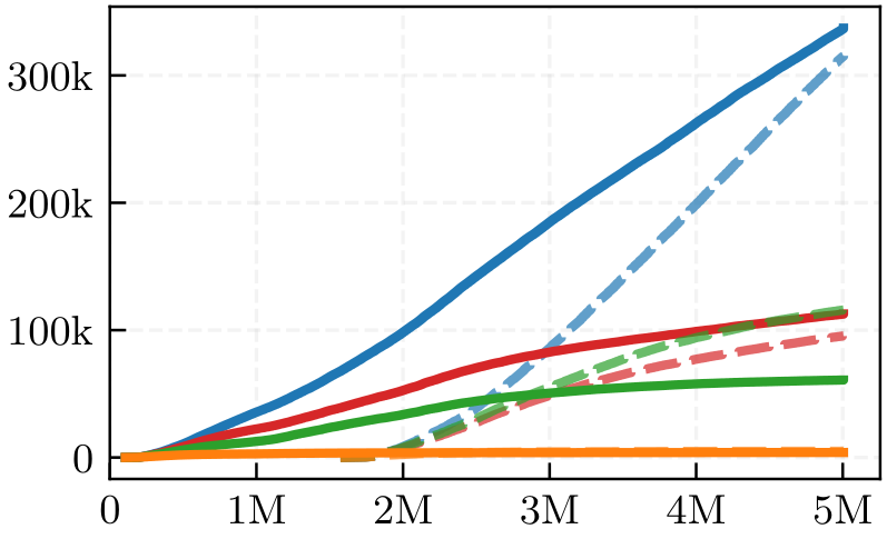
Pre-trained models accelerate discovery times on new geometries. Transferring from a source geometry with a small symmetry group \(|G_{\mathbf{X}_3}|\) to a target with a large \(|G_{\mathbf{X}_3}|\) maintains broad exploration capabilities and yields diverse solution sets.
Transferring from large to small symmetry groups traps the policy in local minima. The network finds the first solution rapidly but fails to accumulate unique line bundle sums efficiently. Similar directional asymmetries occur for shifts in \(h^{1,1}(\mathbf{X}_3)\) and \(|\Gamma|\).
Optimal transfer directions include:
- Small \(|G_{\mathbf{X}_3}|\) to large \(|G_{\mathbf{X}_3}|\)
- Large \(|\Gamma|\) to small \(|\Gamma|\)
- Large \(h^{1,1}(\mathbf{X}_3)\) to small \(h^{1,1}(\mathbf{X}_3)\)
Running the LB-Explorer Pipeline
The codebase handles geometry parsing, transformer training, and physical verification.
Geometry Parsing
Convert the master CICY database into the specific format required by the explorer.
python scripts/create_LB-Explorer_inputs.py \
    --db_path databases/full_cicy_database.json \
    --output_dir cy_geometry_exports
Training the RL Agent
Train the PPO agent to search for line bundle matrices. Execution requires specifying the \(h^{1,1}\) dimension, the database index, the symmetry group order \(\Gamma\), and the maximum integer bounds for the line bundle charges.
python LB-Explorer.py \
    --h11 5 \
    --cy_index 7447 \
    --gamma 2 \
    --m_bound 8 \
    --stability_range 2 \
    --use_minibatches \
    --run_id h11_5_g2__cy7447__s42
CP-SAT Hybrid Closure
For highly constrained geometries, the reinforcement learning agent can search for partial matrices by disabling the exact chiral index sum penalty (--sum_coef 0). Feed these partial solutions into a Constraint Programming SAT solver to systematically find the remaining columns required to close the matrix and satisfy all constraints.
python CPSAT-closure.py \
    --solutions sol_runs_h11_5_g2__cy7447__s42/solutions_gpu_*.jsonl \
    --geometry cy_geometry_exports/all_geometry_h11_5.json \
    --cy_index 7447 \
    --gamma 2
Physics Verification
Process the raw generated matrices through standalone scripts to verify equivariance, exact poly-stability (via SciPy optimization), and compute the explicit bundle cohomologies (via pyCICY).
python scripts/check_validity_solutions.py --rank 5 --input_dir Sol_Runs
python scripts/check_equivariance.py --workers 8
References
[1] D. J. Gross, J. A. Harvey, E. J. Martinec, and R. Rohm, "The Heterotic String", Phys. Rev. Lett. 54, 502--505 (1985).
[2] D. J. Gross, J. A. Harvey, E. J. Martinec, and R. Rohm, "Heterotic String Theory. 1. The Free Heterotic String", Nucl. Phys. B 256, 253 (1985).
[3] D. J. Gross, J. A. Harvey, E. J. Martinec, and R. Rohm, "Heterotic String Theory. 2. The Interacting Heterotic String", Nucl. Phys. B 267, 75--124 (1986).
[4] P. Candelas, G. T. Horowitz, A. Strominger, and E. Witten, "Vacuum configurations for superstrings", Nucl. Phys. B 258, 46--74 (1985).
[5] B. R. Greene, K. H. Kirklin, P. J. Miron, and G. G. Ross, "A Superstring Inspired Standard Model", Phys. Lett. B 180, 69 (1986).
[6] B. R. Greene, K. H. Kirklin, P. J. Miron, and G. G. Ross, "A Three Generation Superstring Model. 1. Compactification and Discrete Symmetries", Nucl. Phys. B 278, 667--693 (1986).
[7] B. R. Greene, K. H. Kirklin, P. J. Miron, and G. G. Ross, "A Three Generation Superstring Model. 2. Symmetry Breaking and the Low-Energy Theory", Nucl. Phys. B 292, 606--652 (1987).
[8] J. Distler and B. R. Greene, "Aspects of (2,0) String Compactifications", Nucl. Phys. B 304, 1--62 (1988).
[9] J. Distler and S. Kachru, "(0,2) Landau-Ginzburg theory", Nucl. Phys. B 413, 213--243 (1994), arXiv:hep-th/9309110.
[10] S. Kachru, "Some three generation (0,2) Calabi-Yau models", Phys. Lett. B 349, 76--82 (1995), arXiv:hep-th/9501131.
[11] L. B. Anderson, A. Constantin, J. Gray, A. Lukas, and E. Palti, "A Comprehensive Scan for Heterotic SU(5) GUT models", JHEP 01, 047 (2014), arXiv:1307.4787.
[12] S. K. Donaldson, "Anti Self-Dual Yang-Mills Connections over Complex Algebraic Surfaces and Stable Vector Bundles", Proc. Lond. Math. Soc. 50, 1--26 (1985).
[13] K. Uhlenbeck and S. T. Yau, "On the existence of hermitian-yang-mills connections in stable vector bundles", Commun. Pure Appl. Math. 39, no. S1, S257--S293 (1986).
[14] L. B. Anderson, J. Gray, A. Lukas, and E. Palti, "Two Hundred Heterotic Standard Models on Smooth Calabi-Yau Threefolds", Phys. Rev. D 84, 106005 (2011), arXiv:1106.4804.
[15] L. B. Anderson, J. Gray, A. Lukas, and E. Palti, "Heterotic Line Bundle Standard Models", JHEP 06, 113 (2012), arXiv:1202.1757.
[16] J. Schulman, F. Wolski, P. Dhariwal, A. Radford, and O. Klimov, "Proximal Policy Optimization Algorithms", arXiv:1707.06347 (2017).
[17] A. Vaswani, N. Shazeer, N. Parmar, J. Uszkoreit, L. Jones, A. N. Gomez, L. Kaiser, and I. Polosukhin, "Attention Is All You Need", arXiv:1706.03762 (2017).
[18] J. Lei Ba, J. R. Kiros, and G. E. Hinton, "Layer Normalization", arXiv:1607.06450 (2016).
[19] X. Glorot and Y. Bengio, "Understanding the difficulty of training deep feedforward neural networks", PMLR 9, 249--256 (2010).
[20] J. Schulman, P. Moritz, S. Levine, M. Jordan, and P. Abbeel, "High-Dimensional Continuous Control Using Generalized Advantage Estimation", arXiv:1506.02438 (2015).
[21] P. Candelas, A. M. Dale, C. A. Lutken, and R. Schimmrigk, "Complete Intersection Calabi-Yau Manifolds", Nucl. Phys. B 298, 493 (1988).
[22] L. B. Anderson, Y.-H. He, and A. Lukas, "Heterotic Compactification, An Algorithmic Approach", JHEP 07, 049 (2007), arXiv:hep-th/0702210.
[23] L. B. Anderson, Y.-H. He, and A. Lukas, "Monad Bundles in Heterotic String Compactifications", JHEP 07, 104 (2008), arXiv:0805.2875.